

Understanding the concepts of total cost, cost categories, average cost, and marginal cost is fundamental in economics, particularly in the study of how businesses operate and make decisions. Let’s explore each concept in detail:
### 1. Total Cost Curve
The total cost curve represents the total economic cost of production as a function of the quantity of output produced. It combines all costs faced by a business, including both fixed and variable costs.
– **Fixed Costs (FC)**: These are costs that do not change with the level of output. They are incurred even when output is zero. Examples include rent, salaries of permanent staff, and depreciation of capital equipment.
– **Variable Costs (VC)**: These costs vary directly with the level of production. The more a firm produces, the higher the variable costs. Examples include raw materials, energy usage, and wages for hourly labor.
The total cost (TC) is the sum of fixed costs and variable costs at any given level of production:
\[ \text{TC} = \text{FC} + \text{VC} \]
Graphically, the total cost curve typically starts at the level of fixed costs (since these are incurred regardless of output) and slopes upwards, reflecting an increase in variable costs as production increases.
### 2. Cost Categories
– **Fixed Costs**: As mentioned, these do not change with output. They are often termed as sunk costs because they remain constant regardless of business activity levels.
– **Variable Costs**: These increase with an increase in output. The relationship might not always be linear, as some variable costs may increase at a decreasing or increasing rate.
– **Semi-variable Costs**: Some costs have both fixed and variable components. For example, electricity might have a minimum charge (fixed), plus a charge per unit of electricity used (variable).
### 3. Average Costs
Average costs are calculated by dividing the total cost (TC) by the quantity of output (Q).
– **Average Total Cost (ATC)**: This is the total cost per unit of output, calculated as:
\[ \text{ATC} = \frac{\text{TC}}{Q} \]
– **Average Fixed Cost (AFC)**: This represents the fixed cost per unit of output and decreases as output increases because the same amount of fixed costs is spread over more units of output.
\[ \text{AFC} = \frac{\text{FC}}{Q} \]
– **Average Variable Cost (AVC)**: This is the variable cost per unit of output.
\[ \text{AVC} = \frac{\text{VC}}{Q} \]
### 4. Marginal Cost
Marginal cost is the additional cost of producing one more unit of output. It is a crucial concept for decision-making in production. Mathematically, it can be approximated by the change in total cost divided by the change in output:
\[ \text{MC} = \frac{\Delta \text{TC}}{\Delta Q} \]
In practical analysis, marginal cost helps determine the optimal level of production. A business may decide to produce additional units as long as the revenue from selling those units exceeds the marginal cost of producing them.
Graphically, the marginal cost curve often intersects the average total cost and average variable cost curves at their lowest points. This intersection is significant because it represents the point of minimum average costs, which is often associated with efficient scales of production in the short run.
Understanding these concepts allows businesses and economists to analyze production efficiency, make cost-effective production decisions, and understand the behavior of cost curves in response to changes in output levels.
Let’s consider a hypothetical company that manufactures widgets and go through a detailed example to illustrate the concepts of fixed costs, variable costs, total costs, average costs, and marginal costs.
### Company Overview:
– **Fixed Costs (FC)**: $1,000 per month (rent, salaries, etc.)
– **Variable Cost (VC)** per widget: $5 (materials, energy, etc.)
### Scenario:
We’ll calculate the costs for producing 0 to 10 widgets to observe how each cost behaves and interacts.
### Step-by-Step Calculation:
1. **Total Cost (TC)** = Fixed Costs (FC) + Variable Costs (VC)
2. **Variable Costs (VC)** = Variable Cost per Unit × Quantity of Widgets
3. **Average Total Cost (ATC)** = Total Cost / Quantity of Widgets
4. **Average Fixed Cost (AFC)** = Fixed Costs / Quantity of Widgets
5. **Average Variable Cost (AVC)** = Variable Costs / Quantity of Widgets
6. **Marginal Cost (MC)** = Change in Total Cost / Change in Quantity
Let’s calculate these costs for quantities from 0 to 10 widgets:
| Quantity (Q) | Fixed Cost (FC) | Variable Cost (VC) | Total Cost (TC) | Average Fixed Cost (AFC) | Average Variable Cost (AVC) | Average Total Cost (ATC) | Marginal Cost (MC) |
|---|---|---|---|---|---|---|---|
| 0 | $1,000 | $0 | $1,000 | – | – | – | – |
| 1 | $1,000 | $5 | $1,005 | $1,000 | $5 | $1,005 | $5 |
| 2 | $1,000 | $10 | $1,010 | $500 | $5 | $505 | $5 |
| 3 | $1,000 | $15 | $1,015 | $333.33 | $5 | $338.33 | $5 |
| 4 | $1,000 | $20 | $1,020 | $250 | $5 | $255 | $5 |
| 5 | $1,000 | $25 | $1,025 | $200 | $5 | $205 | $5 |
| 6 | $1,000 | $30 | $1,030 | $166.67 | $5 | $171.67 | $5 |
| 7 | $1,000 | $35 | $1,035 | $142.86 | $5 | $147.86 | $5 |
| 8 | $1,000 | $40 | $1,040 | $125 | $5 | $130 | $5 |
| 9 | $1,000 | $45 | $1,045 | $111.11 | $5 | $116.11 | $5 |
| 10 | $1,000 | $50 | $1,050 | $100 | $5 | $105 | $5 |
### Observations:
– **Fixed Cost (FC)** remains constant at $1,000 regardless of production.
– **Variable Cost (VC)** increases linearly by $5 for each additional widget produced.
– **Total Cost (TC)** starts at $1,000 (when no widgets are produced) and increases by $5 for each additional widget.
– **Average Fixed Cost (AFC)** decreases as production increases because the fixed cost is spread over more units.
– **Average Variable Cost (AVC)** remains constant at $5 per widget, reflecting the constant variable cost per unit.
– **Average Total Cost (ATC)** starts very high when production is low due to high fixed costs per unit but decreases as more widgets are produced.
– **Marginal Cost (MC)** remains constant at $5, equal to the increase in variable costs for each additional widget.
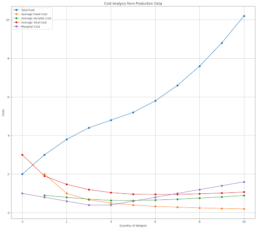
Let’s see a more complex example with its graph:
| Quantity (Q) | Total Cost (TC) | Fixed Cost (FC) | Variable Cost (VC) | Average Fixed Cost (AFC) | Average Variable Cost (AVC) | Average Total Cost (ATC) | Marginal Cost (MC) |
|---|---|---|---|---|---|---|---|
| 0 | 2.00 | 2.00 | 0.00 | – | – | 3.00 | 1.00 |
| 1 | 3.00 | 2.00 | 1.00 | 2.00 | 0.90 | 1.90 | 0.80 |
| 2 | 3.80 | 2.00 | 1.80 | 1.00 | 0.80 | 1.47 | 0.60 |
| 3 | 4.40 | 2.00 | 2.40 | 0.67 | 0.70 | 1.20 | 0.40 |
| 4 | 4.80 | 2.00 | 2.80 | 0.50 | 0.64 | 1.04 | 0.40 |
| 5 | 5.20 | 2.00 | 3.20 | 0.40 | 0.63 | 0.96 | 0.60 |
| 6 | 5.80 | 2.00 | 3.80 | 0.33 | 0.66 | 0.95 | 0.80 |
| 7 | 6.60 | 2.00 | 4.60 | 0.29 | 0.70 | 0.95 | 1.00 |
| 8 | 7.60 | 2.00 | 5.60 | 0.25 | 0.76 | 0.98 | 1.20 |
| 9 | 8.80 | 2.00 | 6.80 | 0.22 | 0.82 | 1.02 | 1.40 |
| 10 | 10.20 | 2.00 | 8.20 | 0.20 | 0.89 | 1.07 | 1.60 |
The second table provides a detailed breakdown of various cost metrics across different production levels for widgets. Here are some key observations from the data:
1. **Fixed Costs Remain Constant**: As expected, the Fixed Cost (FC) remains constant at 2.00 across all production levels, illustrating that these costs are not affected by the volume of output.
2. **Increase in Variable Costs**: The Variable Cost (VC) increases with the quantity of output, reflecting the additional resources required for each additional unit produced. This increase is incremental and becomes more pronounced as production scales up.
3. **Decrease in Average Fixed Costs**: The Average Fixed Cost (AFC) consistently decreases as production increases. This is due to the fixed cost being spread over a larger number of units, thus reducing the cost per unit.
4. **Variable Trend in Average Variable Costs**: The Average Variable Cost (AVC) generally increases, suggesting that additional units are becoming more expensive to produce. This could be due to factors such as the use of more costly materials or less efficient labor as production is pushed beyond optimal capacity.
5. **Marginal Cost Increases**: The Marginal Cost (MC) starts low and increases with production. This increase highlights that producing additional units becomes progressively more expensive, which is often due to reaching capacity limits or inefficiencies that arise from scaling production.
6. **Total and Average Total Costs**: The Total Cost (TC) and Average Total Cost (ATC) both increase as more units are produced. Notably, the ATC first decreases, reaching its lowest point around a production level of 7 units, before starting to increase again. This is a typical representation of the “U-shaped” ATC curve in economics, where costs per unit decrease up to a point due to economies of scale before increasing due to diseconomies of scale.
7. **Optimal Production Level**: The lowest ATC is observed at a production level of 7 units, suggesting this might be the most cost-efficient production point under current cost conditions.
These observations provide valuable insights into the cost behavior of production and can inform decisions regarding optimal production levels, pricing strategies, and potential adjustments to cost structures to enhance profitability.
The examples above integrate these cost concepts and demonstrate how they interrelate in the context of production decisions.