Comprehensive Article on the Geometric and Negative Binomial Distributions

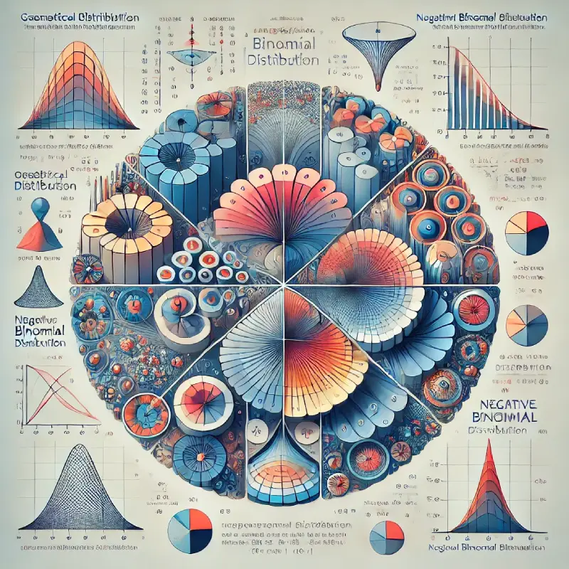
Comprehensive Article on the Geometric and Negative Binomial Distributions

Introduction

In probability theory, the Geometric and Negative Binomial distributions are two closely related discrete distributions. Both are used to model the number of trials required to achieve a certain number of successes in independent Bernoulli trials. These distributions are powerful tools in various applications, ranging from quality control to survival analysis. This article provides an expansive overview of the Geometric and Negative Binomial distributions, exploring their definitions, properties, applications, and interconnections.

—

The Geometric Distribution

1. Definition

The Geometric distribution models the number of trials required to achieve the first success in a sequence of independent and identically distributed Bernoulli trials. In each trial, there are two possible outcomes: success (with probability \( p \)) or failure (with probability \( 1-p \)).

2. Mathematical Representation

If \( X \) denotes the random variable representing the number of trials until the first success, then \( X \) follows a Geometric distribution with parameter \( p \). The probability mass function (PMF) is given by:

\[
P(X = k) = (1-p)^{k-1} p \quad \text{for} \quad k = 1, 2, 3, \dots
\]

Here, \( k \) represents the number of trials needed to get the first success.

3. Key Properties

– Mean (Expected Value): The expected number of trials to get the first success is \( \text{E}[X] = \frac{1}{p} \).
– Variance: The variance of the Geometric distribution is \( \text{Var}(X) = \frac{1-p}{p^2} \).
– Memoryless Property: One unique feature of the Geometric distribution is its memorylessness. This means that the probability of success in future trials does not depend on the number of failures so far. Mathematically, for any \( m \) and \( n \):

\[
P(X > m + n \mid X > m) = P(X > n)
\]

This property is not shared by many other distributions and makes the Geometric distribution particularly interesting.

4. Applications of the Geometric Distribution

– Modeling Time Until an Event: The Geometric distribution is widely used to model the number of attempts required for a single event to occur. For example, in customer service, it can model the number of calls needed to reach the first successful sales pitch.
– Reliability Testing: It can be used to model the number of cycles or time intervals before a system or component fails.
– Clinical Trials: The distribution is useful in determining the number of patients needed to observe the first successful outcome in a trial.

—

The Negative Binomial Distribution

1. Definition

The Negative Binomial distribution generalizes the Geometric distribution to model the number of trials required to achieve a specified number of successes in a sequence of independent Bernoulli trials. Instead of stopping after the first success, the process continues until a fixed number of successes \( r \) is observed.

2. Mathematical Representation

Let \( Y \) denote the random variable representing the number of trials needed to achieve \( r \) successes, with \( r \) being a positive integer and \( p \) the probability of success on each trial. The PMF of the Negative Binomial distribution is given by:

\[
P(Y = k) = \binom{k-1}{r-1} p^r (1-p)^{k-r} \quad \text{for} \quad k = r, r+1, r+2, \dots
\]

Here, \( k \) represents the number of trials required to achieve \( r \) successes.

3. Key Properties

– Mean (Expected Value): The mean of the Negative Binomial distribution is \( \text{E}[Y] = \frac{r}{p} \).
– Variance: The variance is \( \text{Var}(Y) = \frac{r(1-p)}{p^2} \).
– Relationship to Geometric Distribution: When \( r = 1 \), the Negative Binomial distribution reduces to the Geometric distribution.

4. Applications of the Negative Binomial Distribution

– Count Data Modeling: The Negative Binomial distribution is often used to model overdispersed count data, where the variance exceeds the mean, such as the number of accidents occurring at an intersection over a period of time.
– Genetics and Ecology: It is used to model the number of occurrences of specific traits or events in populations, such as the number of rare species found in a set of ecological samples.
– Banking and Finance: The distribution can model the number of defaults before a certain number of loans are repaid successfully, which is useful in risk assessment.

—

Interconnection Between Geometric and Negative Binomial Distributions

The Geometric and Negative Binomial distributions are inherently connected, as the latter generalizes the former. The Geometric distribution is essentially a special case of the Negative Binomial distribution with \( r = 1 \). This means that the Geometric distribution can be viewed as a Negative Binomial distribution where the number of successes required is exactly one.

1. Deriving Geometric from Negative Binomial

Given the PMF of the Negative Binomial distribution:

\[
P(Y = k) = \binom{k-1}{r-1} p^r (1-p)^{k-r}
\]

When \( r = 1 \), this simplifies to:

\[
P(X = k) = (1-p)^{k-1} p
\]

which is the PMF of the Geometric distribution.

2. Applications in Real-World Scenarios

Both distributions are valuable in scenarios where repeated trials are observed until one or more successes occur. In reliability engineering, the Geometric distribution can model the number of operational cycles before a machine part fails (first success), while the Negative Binomial distribution can model the number of cycles before a certain number of parts fail.

—

Conclusion

The Geometric and Negative Binomial distributions are fundamental discrete distributions in probability theory, particularly useful in modeling scenarios involving repeated trials with binary outcomes. The Geometric distribution focuses on the trials needed to achieve the first success, while the Negative Binomial distribution generalizes this to the trials needed for multiple successes.

Understanding these distributions and their properties is crucial for analyzing processes where the timing or frequency of successes matters. Their applications are vast, ranging from quality control and risk management to ecological studies and customer behavior modeling. By leveraging these distributions, statisticians and analysts can gain deeper insights into the underlying processes governing random events.