Introduction
In economics, understanding the cost structure and profitability of firms in a competitive market is essential. This knowledge helps in analyzing how firms make decisions about production, pricing, and market entry or exit. This article delves into the long-run supply curve of a competitive firm, explaining key concepts such as marginal cost, average total cost, and the conditions under which firms earn profits, break even, or incur losses.
The Long-Run Supply Curve
Marginal Cost (MC) and Average Total Cost (ATC)
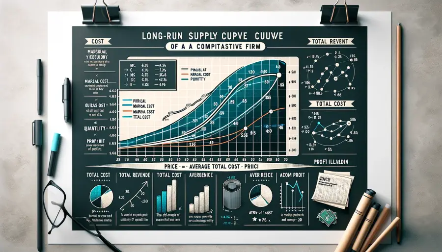
The long-run supply curve of a competitive firm is primarily determined by two cost curves: the Marginal Cost (MC) curve and the Average Total Cost (ATC) curve.
- Marginal Cost (MC): This curve represents the additional cost incurred by producing one more unit of output. It is a crucial concept because it influences the firm’s production decisions. In the long run, firms adjust all their inputs, making the MC curve a key indicator of how production costs change with varying levels of output.
- Average Total Cost (ATC): This curve shows the average cost of production per unit, incorporating both fixed and variable costs. The ATC curve helps in understanding the overall efficiency and cost structure of the firm.
The Supply Curve in the Long Run
In a competitive market, the supply curve of a firm in the long run is the portion of the MC curve that lies above the ATC curve. Here’s why:
- Profitability and Production Decisions: For a firm to produce in the long run, the price (P) at which it sells its product must be higher than the ATC. This ensures that the firm can cover all its costs, including both fixed and variable costs. If the price is below the ATC, the firm would incur losses and eventually exit the market.
- Market Equilibrium: In the long run, firms will only supply quantities of their product where the price is at least equal to the ATC. Therefore, the long-run supply curve is the segment of the MC curve above the ATC curve.
Profit Calculation
Total Revenue and Total Cost
To understand a firm’s profitability, we look at the relationship between Total Revenue (TR) and Total Cost (TC):
- Total Revenue (TR): This is the total income a firm receives from selling its product. It is calculated as the price per unit (P) multiplied by the quantity sold (Q):
\[
TR = P \times Q
\] - Total Cost (TC): This is the total expenditure incurred in producing the product. It includes all fixed and variable costs.
Profit Formula
Profit is the difference between Total Revenue and Total Cost:
\[
\text{Profit} = TR – TC
\]
This formula can be further analyzed by breaking it down into per-unit costs and revenues:
- Average Revenue (AR): In a competitive market, the average revenue per unit is equal to the price (P).
- Average Total Cost (ATC): This is the total cost per unit produced.
We can rewrite the profit formula by dividing and multiplying it by the quantity (Q):
\[
\text{Profit} = (TR/Q – TC/Q) \times Q
\]
Since (TR/Q) is the average revenue (P), and (TC/Q) is the average total cost (ATC), the formula becomes:
\[
\text{Profit} = (P – ATC) \times Q
\]
Interpretation of the Profit Formula
This formula indicates that the profit per unit is the difference between the price and the average total cost, multiplied by the quantity produced and sold. This interpretation leads to several important insights:
- Break-Even Point: The firm breaks even when the price equals the average total cost (P = ATC). At this point, the firm’s total revenue equals its total cost, resulting in zero economic profit.
- Profit: The firm earns a profit when the price is greater than the average total cost (P > ATC). In this scenario, the revenue per unit exceeds the cost per unit, leading to a positive profit.
- Loss: Conversely, the firm incurs a loss when the price is less than the average total cost (P < ATC). Here, the cost per unit exceeds the revenue per unit, resulting in negative profit.
Long-Run Market Dynamics
Entry and Exit of Firms
In the long run, the market dynamics are influenced by the entry and exit of firms based on profitability:
- Entry: If existing firms are earning economic profits (P > ATC), new firms are attracted to the market. The entry of new firms increases the market supply, which can lead to a decrease in the market price.
- Exit: If existing firms are incurring losses (P < ATC), some firms will exit the market. The exit of firms decreases the market supply, which can lead to an increase in the market price.
Long-Run Equilibrium
In the long run, the competitive market reaches an equilibrium where firms earn zero economic profit (P = ATC). At this point, no new firms enter or exit the market, and the price stabilizes. This equilibrium ensures that firms cover all their costs, including a normal profit (the minimum return necessary to keep resources in their current use).
Conclusion
The long-run supply curve of a competitive firm is a crucial concept in economics, reflecting how firms make production decisions based on costs and market prices. By understanding the relationship between marginal cost, average total cost, and market price, we can analyze how firms achieve profitability, break even, or incur losses. The dynamics of entry and exit in response to profitability ensure that competitive markets tend towards a long-run equilibrium where firms earn zero economic profit. This equilibrium state highlights the efficiency and self-regulating nature of competitive markets.
This comprehensive article provides an in-depth analysis of the long-run supply curve of a competitive firm, elucidating the fundamental economic principles that govern firm behavior and market dynamics.

